[Machine Learning] Multiclass Classification

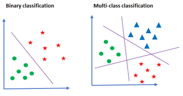
Multi-class Classification

• LogisticRegression classifier():
• OvR and softmax classifier
• In the multiclass case, the training algorithm uses the one-vs-rest (OvR) scheme if the ‘multi_class’ option is set to ‘ovr’, and uses the softmax (with cross-entropy) if the ‘multi_class’ option is set to ‘multinomial’.

Classifier

OvR (One versus Rest)

OvR이란 이름에서 알 수 있듯이 분류 클래스 중 하나와 나머지를 분류하는 것을 여러 번 수행하여 다중 분류를 수행하는 것입니다.

이는 다중 분류를 위해 이중 분류를 사용하는 휴리스틱적인 방법이라고 할 수 있습니다.

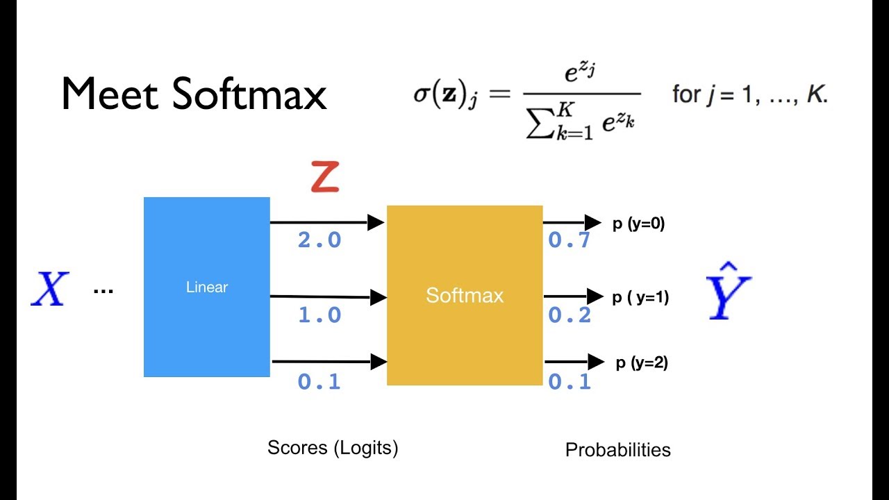
Softmax

Softmax란 다중 분류에서 사용되는 활성화 함수입니다.

이중 분류에서는 각 클래스에 속할 점수를 Sigmoid 함수를 사용하여 확률로 변환한 것과 같이, 다중 분류에서는 각 클래스에 속할 점수를 Softmax 함수를 사용하여 확률로 변환합니다.

여기서 다른 활성화 함수를 사용하는 이유는 확률은 각 클래스에 속할 점수의 합이 1이 되어야 하기 때문입니다.

Setup

import numpy as np
import pandas as pd
import matplotlib.pyplot as plt
%matplotlib inline
from sklearn import datasets
from sklearn.model_selection import train_test_split
from sklearn.linear_model import SGDClassifier, LogisticRegression
from sklearn import metrics
from sklearn.model_selection import cross_val_score, KFold

two features

시각적으로 확인하기 위해 먼저 두 개의 특성으로 다중 분류 수행

iris = datasets.load_iris()
X, y = iris.data[:,(2,3)], iris.target

LogisticRegression에 multi_class="multinomial" 또는 multi_class="ovr"을 하이퍼 파라미터로 지정하여 다중 분류를 수행할 수 있다.

• "multinomial": 다중 분류로 softmax 사용
• "ovr": 다중 분류로 OvR(One vs Rest) 사용

softmax_reg = LogisticRegression(multi_class="multinomial", C=10, random_state=42)
ovr_clf = LogisticRegression(multi_class="ovr", C=10, random_state=42)
softmax_reg.fit(X, y)
ovr_clf.fit(X, y)

LogisticRegression(C=10, multi_class='ovr', random_state=42)

모델 평가

softmax_reg.score(X, y), ovr_clf.score(X, y)

(0.96, 0.96)

모델의 파라미터 확인

softmax_reg.coef_, softmax_reg.intercept_

(array([[-4.58614563, -2.24129385],
        [ 0.16068263, -2.15860167],
        [ 4.425463  ,  4.39989552]]),
 array([ 18.87514796,   6.3844344 , -25.25958236]))

ovr_clf.coef_, ovr_clf.intercept_

(array([[-4.10145565, -1.8601741 ],
        [ 1.42847909, -2.83149429],
        [ 4.42142146,  5.74004612]]),
 array([ 12.11411097,  -2.73490959, -31.06624834]))

분류 확인

x0, x1 = np.meshgrid(
        np.linspace(0, 8, 500).reshape(-1, 1),
        np.linspace(0, 3.5, 200).reshape(-1, 1),
    )
X_new = np.c_[x0.ravel(), x1.ravel()]

y_proba = softmax_reg.predict_proba(X_new)
y_predict = softmax_reg.predict(X_new)

zz1 = y_proba[:, 1].reshape(x0.shape)
# zz2 = y_proba[:, 2].reshape(x0.shape)
zz = y_predict.reshape(x0.shape)

plt.figure(figsize=(10, 4))
plt.plot(X[y==2, 0], X[y==2, 1], "g^", label="Iris virginica")
plt.plot(X[y==1, 0], X[y==1, 1], "bs", label="Iris versicolor")
plt.plot(X[y==0, 0], X[y==0, 1], "yo", label="Iris setosa")

from matplotlib.colors import ListedColormap
custom_cmap = ListedColormap(['#fafab0','#9898ff','#a0faa0'])

plt.contourf(x0, x1, zz, cmap=custom_cmap)
contour = plt.contour(x0, x1, zz1, cmap=plt.cm.brg)
plt.clabel(contour, fontsize=12)
plt.xlabel("Petal length", fontsize=14)
plt.ylabel("Petal width", fontsize=14)
plt.legend(loc="center left", fontsize=14)
plt.axis([0, 7, 0, 3.5])

plt.show()
    

예측 수행

softmax_reg.predict([[5, 2]])

array([2])

softmax_reg.predict_proba([[5, 2]])

array([[6.38014896e-07, 5.74929995e-02, 9.42506362e-01]])

four features

전체 feature에 대해 다중 분류 수행

iris = datasets.load_iris()
X, y = iris.data, iris.target
X_train, X_test, y_train, y_test = train_test_split(X, y, test_size=0.3)

clf_all = SGDClassifier(max_iter=1000)
clf_all.fit(X_train, y_train)
clf_all.score(X_test, y_test)

0.9333333333333333

softmax_reg.fit(X_train, y_train)
softmax_reg.score(X_test, y_test)

0.9777777777777777

ovr_clf.fit(X_train, y_train)
ovr_clf.score(X_test, y_test)

0.9555555555555556

confusion matrix

talk about it later

y_pred = clf_all.predict(X_test)
from sklearn import metrics      # import the metrics class
metrics.confusion_matrix(y_test, y_pred)

array([[13,  4,  0],
       [ 0, 10,  1],
       [ 0, 12,  5]], dtype=int64)

교차 검증

cv = KFold(5,shuffle=True)
scores = cross_val_score(clf_all, X, y, cv=cv)
print(scores)
scores.mean()
# print(cross_val_score(SGDClassifier(), X, y, cv=cv))

[0.8        0.6        0.86666667 0.96666667 0.93333333]

0.8333333333333334

정리

이진 분류와 마찬가지로 다중 분류를 위한 모델에도 LogisticRegression과 SGDClassifier를 사용할 수 있습니다.

LogisticRegression 모델의 경우 기본적으로 회귀와 시그모이드 함수를 사용하기 때문에, 다중 분류를 위해서는 옵션을 주어야 합니다.

이 때 하이퍼 파라미터 multi_class 의 값으로 "ovr" 또는 "multinomial"을 지정할 수 있습니다.

“ovr” 은 OvR(One versus Rest) 방식으로 분류를 수행하고, “multinomial”은 cross entropy + softmax 방식으로 분류를 수행합니다.

SGDClassifier 모델의 경우 기본적으로 분류 모델이기 때문에 하이퍼 파라미터를 지정해주지 않아도 됩니다.

Default 값으로 hinge로 지정되어 있어서 hinge loss를 사용(hinge loss에 대한 설명은 이전 포스팅에 있습니다)하며, log로 값을 지정 시 cross entropy loss를 사용할 수 있습니다. 이외에도 다양한 손실 함수들을 지정할 수 있습니다.