[Machine Learning] Midterm Summary 2
week 6
Imbalance Problem
SMOTE (Synthetic Minority Oversampling TEchnique)
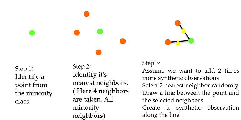

Making imbalance dataset
make_classification: n_samples, n_features, n_redundant, n_clusters_per_classes, weights, flip_y, random_state- n_samples: number of samples
- n_features: number of features
- n_redundant: number of redundant features
- n_classes: number of classes(labels)
- n_clusters_per_class: number of clusters per class
- weights: proportion of samples assigned to each class
- flip_y: fraction of samples whose class is assigned randomly. Larger values introduce noise in the labels and make the classification task harder.
from sklearn.datasets import make_classification
# Highly imbalanced dataset
X_org, y_org = make_classification(n_samples=10000, n_features=2, n_redundant=0,
	                       n_clusters_per_class=1, weights=[0.99], flip_y=0,
                           random_state=1)

def print_result(X_train, X_test, y_train, y_test):

    model = RandomForestClassifier(n_estimators=100, max_depth=5)
    print("Shapes: ", X_train.shape, X_test.shape, y_train.shape, y_test.shape)
    model.fit(X_train, y_train)

    y_pred = model.predict(X_test)
    print("Static performance: ", "\n", confusion_matrix(y_test, y_pred))
    print()
    print(classification_report(y_test, y_pred))

    y_pred_proba = model.predict_proba(X_test)
    fpr, tpr, _ = roc_curve(y_test, y_pred_proba[:,1])
    print("AUC score: ", auc(fpr, tpr))
    print()

X, y = X_org.copy(), y_org.copy()
X_train, X_test, y_train, y_test = train_test_split(X, y, test_size=0.3, stratify=y)
print_result(X_train, X_test, y_train, y_test)

''' Bad recall-1 score!!! Minority class에 대해 현저히 낮은 성능을 보인다.
Shapes:  (7000, 2) (3000, 2) (7000,) (3000,)
Static performance:
 [[2969    1]
 [  18   12]]

              precision    recall  f1-score   support

           0       0.99      1.00      1.00      2970
           1       0.92      0.40      0.56        30

    accuracy                           0.99      3000
   macro avg       0.96      0.70      0.78      3000
weighted avg       0.99      0.99      0.99      3000

AUC score:  0.9161672278338945
'''
Smoted dataset (Oversampling, Resampling)
over_sampling.SMOTE: sampling_strategy, k_neighbors, random_state- fit_resample: X, y
from imblearn.over_sampling import SMOTE

oversample = SMOTE()
X, y = oversample.fit_resample(X_org, y_org)

Undersampled dataset
under_sampling.RandomUnderSampler: sampling_strategy, random_state- fit_resample: X, y
from imblearn.under_sampling import RandomUnderSampler

under = RandomUnderSampler()
X, y = under.fit_resample(X_org, y_org)

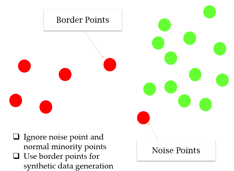
Borderline-SMOTE
Borderline_SMOTE는 Majority class와 Minority class의 샘플의 비율이 비슷한 구역에서만 새로운 sample을 생성함으로써 noise를 무시할 수 있다.

BorderlineSMOTE: sampling_strategy, k_neighbors, m_neighbors, random_state
from imblearn.over_sampling import BorderlineSMOTE

oversample = BorderlineSMOTE(sampling_strategy=0.1)
X, y = oversample.fit_resample(X_org, y_org)

주의할 점!!!
Resampling은 Train set에 대해서만 이루어지고 Test set에는 실제 데이터만이 있어야 한다.
Lab2: Server-based Machine Learning Deployment
# 모델 저장
import pickle

pickle.dump(model, open("파일 경로.pkl", "wb"))
pickle.load(open("파일 경로.pkl", "rb"))

# 웹 페이지 랜더링
from flask import Flask, request, jsonify, render_template

Flask(__name__, template_folder)
- one_off.py
- 입력이 들어오면 바로 추론 값을 반환
- batch_app.py
- 입력이 들어오면 바로 추론 값을 반환하되, 입력을 따로 저장
- 따로 저장한 입력이 일정 개수 이상이 되면 그 데이터들을 이용해 재학습
- 재학습된 모델을 저장
- real_time.py
- 입력이 들어오면 바로 추론 값을 반환하되, 매 입력마다 재학습
- 재학습된 모델을 저장
week 7
OVR (One vs Rest)
n개의 클래스에 대하여 하나의 클래스와 나머지 클래스를 구분하는 것을 n번 반복하여 n개의 클래스를 구분.
OneVsRestClassifier: model
from sklearn.multiclass import OneVsRestClassifier

# SVC uses one-vs-one
classifier = OneVsRestClassifier(SVC(kernel='rbf', C=1000, gamma=0.1, probability=True)) # enable prob estimates
classifier = classifier.fit(X_train, y_train)
SVM
SVC (Classifier)
-
Hinge loss

-
SVC: kernel, degree, C, gamma, probability- kernel: linear, poly, rbf, sigmoid, precomputed (default=rbf)
- degree: degree of the polynomial kernel function (Ignored by all other kernels)
- C: inverse of regularization (값이 커지면 규제가 작아지고 즉, 모델의 복잡도가 증가(노이즈에 민감, 과적합 위험))
- gamma: inverse of deviation (값이 커지면 이웃으로 생각하는 범위가 좁아짐). ‘auto’ = 1 / n_features
- probability: Whether to enable probability estimates.
from sklearn.svm import SVC

svm_clf = SVC(kernel="linear", C=10)
svm_clf.fit(X_train, y_train)
svm_clf = SVC(kernel='rbf', C=1000, gamma=0.1, probability=True)
svm_clf.fit(X_train, y_train)
svm_clf = SVC(kernel='poly', degree=3, C=100, gamma=0.1, probability=True)
svm_clf.fit(X_train, y_train)
C and gamma
For train set

For test set

SVR (Regressor)
-
Epsilon-insenesitive loss

-
SVR: kernel, degree, C, gamma, epsilon- kernel: linear, poly, rbf, sigmoid, precomputed (default=rbf)
- degree: degree of the polynomial kernel function (Ignored by all other kernels)
- C: inverse of regularization (값이 커지면 규제가 작아지고 즉, 모델의 복잡도가 증가(노이즈에 민감, 과적합 위험))
- gamma: inverse of deviation (값이 커지면 이웃으로 생각하는 범위가 좁아짐). ‘auto’ = 1 / n_features
- epsilon: training loss with points predicted within a distance epsilon from the actual value (epslion이 커지면 올바른 예측이라고 여겨지는 street의 너비가 넓어지고 즉, 오차에 관대해진다(모델의 복잡도 감소))
from sklearn.svm import SVR

svr1 = SVR(kernel='linear', epsilon=0.1).fit(x, y)
svr2 = SVR(epsilon=0.01).fit(x, y)
svr3 = SVR(epsilon=1.).fit(x, y)

f, axarr = plt.subplots(1, 3, sharex='col', sharey='row', figsize=(14, 6))

for idx, svr_n, tt in zip(range(3),
                          [svr1, svr2, svr3],
                          ['linear, epsilon=0.1', 'rbf, epsilon=0.01','rbf, epsilon=1.0']):

    axarr[idx].scatter(x, y, s=5, color="blue", label="original")
    yfit = svr_n.predict(x)
    axarr[idx].plot(x, yfit, lw=2, color="red")
    axarr[idx].set_title(tt)

plt.show()

print (svr1.score(x, y), svr2.score(x, y), svr3.score(x, y))

KNN(K Nearest Neighbors)
KNN 은 테스트 시에 새로운 데이터와 인접 데이터들 간의 거리를 계산한다.
따라서 특이하게, 훈련 시에는 하는 것이 없고 테스트 시에 시간이 오래 걸린다.

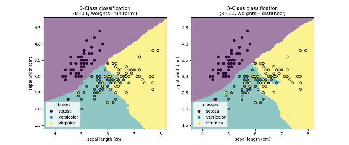
KNN: n_neighbors, weights- n_neighbors: Number of neighbors to use by default for kneighbors queries.
- weights: Weight function use in prediction.
from sklearn.neighbors import KNeighborsClassifier

X_train, X_test, y_train, y_test = train_test_split(X, y, test_size=0.3)

knn = KNeighborsClassifier(n_neighbors=3)
knn.fit(X_train, y_train)
print("kNN score: {:.2f}".format(knn.score(X_test, y_test))) # kNN score: 0.98
Decision Tree
- 모든 feature를 사용해서 나눠보고 가장 잘 구분하는 feature를 사용하여 최종 구분
- 그리디 알고리즘: 당장의 최선의 결정을 선택
- 손실 함수: Impurity (불순도)
- 지니 계수: [0, 0.5] 의 값
- 엔트로피: (-INF, 1] 사이의 값
Classifier
DecisionTreeClassifier: max_depth, min_samples_split, min_samples_leaf, max_features, max_leaf_nodes- max_depth: The maximum depth of tree.
- min_samples_split: The minimum number of samples to split and internal node.
- min_samples_leaf: The minimum number of samples required to be at a leaf node.
- max_features: The number of features to consider when looking for the best split.
- max_leaf_nodes: The maximum number of leaf nodes of tree.
from sklearn.tree import DecisionTreeClassifier
clf = DecisionTreeClassifier(max_depth=2)
clf.fit(X, y)
clf.score(X, y)
tree.plot_tree: tree model, filled
from sklearn import tree

tree.plot_tree(clf, filled=True) # filled=True -> paint to indicate majority class

%matplotlib inline
import matplotlib.pyplot as plt
import numpy as np

plt.xlim(4, 8.5)
plt.ylim(1.5, 4.5)

markers = ['o', '+', '^']
for i in range(3):
    xs = X[:, 0][y == i]
    ys = X[:, 1][y == i]
    plt.scatter(xs, ys, marker=markers[i])

plt.legend(iris.target_names)
plt.xlabel("Sepal length")
plt.ylabel("Sepal width")


# 결정 트리 경계선: 실선은 루트 노드 점선은 자식 노드
xx = np.linspace(5.45, 5.45, 3)
yy = np.linspace(1.5, 4.5, 3)
plt.plot(xx, yy, '-k') # 검정색 실선

xx = np.linspace(4, 5.45, 3)
yy = np.linspace(2.8, 2.8, 3)
plt.plot(xx, yy, '--b') # 파란색 점선

xx = np.linspace(6.15, 6.15, 3)
yy = np.linspace(1.5, 4.5, 3)
plt.plot(xx, yy, '--r') # 붉은색 점선

Regressor
DecisionTreeRegressor: max_depth, min_samples_split, min_samples_leaf, max_features, max_leaf_nodes
from sklearn.tree import DecisionTreeRegressor

X = iris.data[:,:2]
y = iris.data[:,2]
X_train, X_test, y_train, y_test = train_test_split(X, y, test_size=0.2)

tr_reg1 = DecisionTreeRegressor(max_depth=2)
tr_reg1.fit(X_train,y_train)
tr_reg1.score(X_test, y_test)


Ensemble
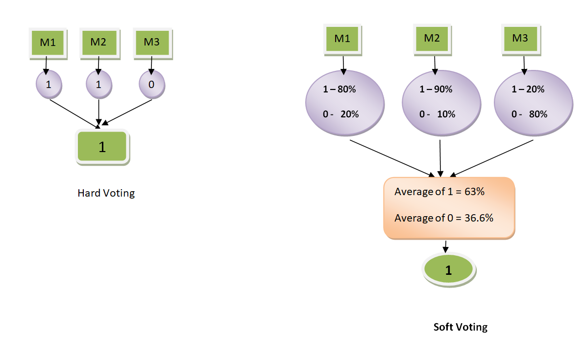
Voting (Stacking)
- Hard Voting: 가장 많은 모델이 예측한 클래스로 최종 결정
- Soft Voting: 각 모델이 예측한 각 클래스의 확률을 고려, 각 클래스 별로 평균하여 최종 결정
VotingClassifier: estimators, voting, weights
from sklearn.ensemble import VotingClassifier

clf1 = LogisticRegression(multi_class='multinomial', random_state=1)
clf2 = RandomForestClassifier(n_estimators=50, random_state=1)
clf3 = GaussianNB()

X = np.array([[-1, -1], [-2, -1], [-3, -2], [1, 1], [2, 1], [3, 2]])
y = np.array([1, 1, 1, 2, 2, 2])

eclf1 = VotingClassifier(estimators=[
         ('lr', clf1), ('rf', clf2), ('gnb', clf3)], voting='hard')
eclf1 = eclf1.fit(X, y)
print(eclf1.predict(X)) # [1 1 1 2 2 2]
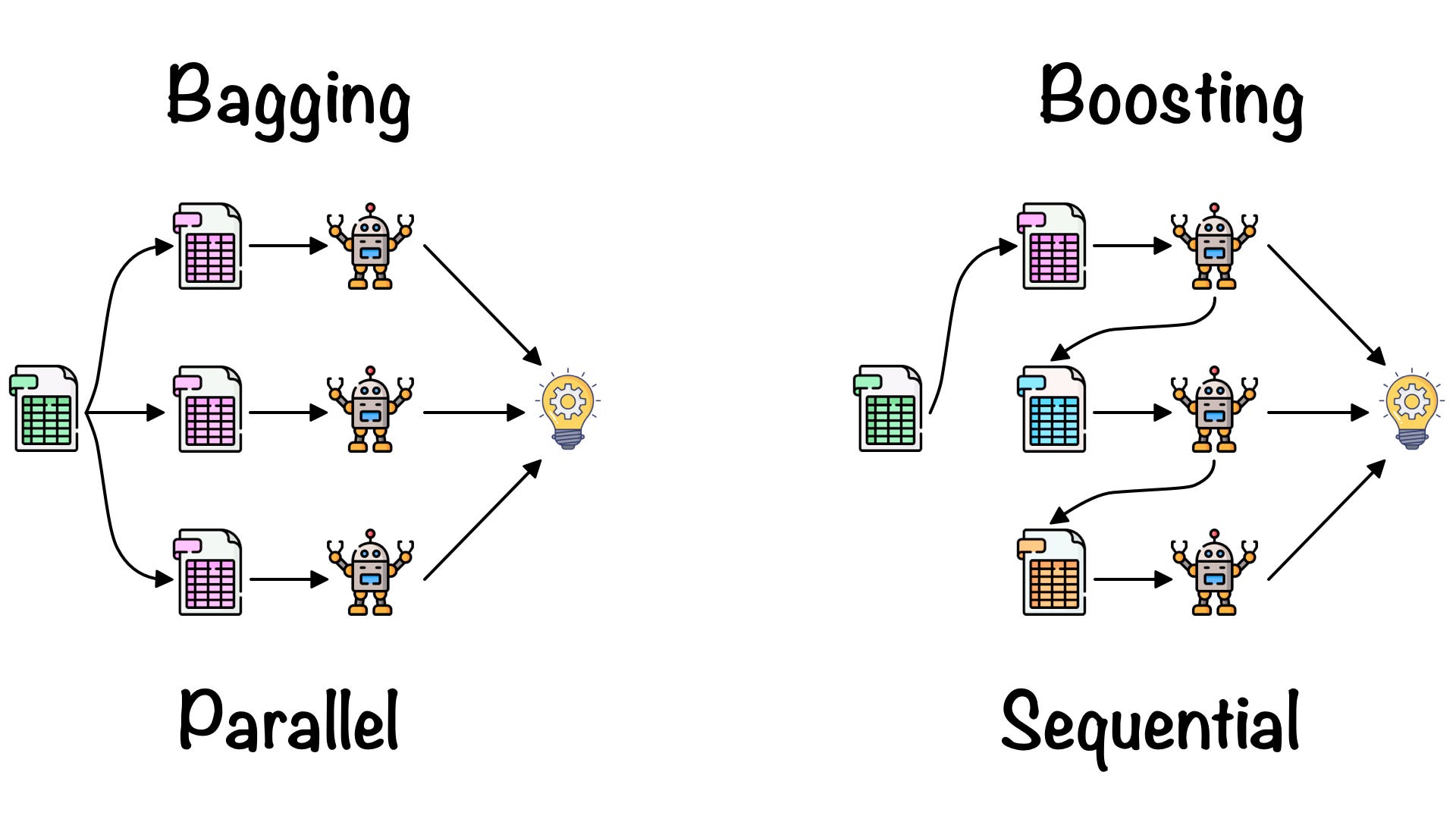
RandomForest (Bagging)
- 중복을 허용한 n개의 샘플을 추출하여 평균을 구하는 작업을 n번 반복
- Overfitting 해소, 일반적인 모델 생성
- Parallel Session
|  |
RandomForestClassifier/RandomForestRegressor: n_estimators, max_depth, min_samples_split, min_samples_leaf, max_features, max_leaf_nodes
from sklearn.ensemble import RandomForestClassifier

cancer = load_breast_cancer()
np.random.seed(9)
X_train, X_test, y_train, y_test = train_test_split(
    cancer.data, cancer.target, stratify=cancer.target)

rfc = RandomForestClassifier(n_estimators=500)
rfc.fit(X_train, y_train)
print(rfc.score(X_test, y_test))

# feature_importances_
list(zip(cancer.feature_names, rfc.feature_importances_.round(4)))[:10]
'''
[('mean radius', 0.0),
 ('mean texture', 0.0417),
 ('mean perimeter', 0.0),
 ('mean area', 0.0),
 ('mean smoothness', 0.0),
 ('mean compactness', 0.0),
 ('mean concavity', 0.0),
 ('mean concave points', 0.0426),
 ('mean symmetry', 0.0114),
 ('mean fractal dimension', 0.0)]
'''
Boosting
- Bagging은 독립적인 input data를 가지고(복원 추출) 독립적으로 예측하지만, Boosting은 이전 모델이 다음 모델에 영향을 준다.
- 맞추기 어려운 문제를 맞추는 것에 초점을 둔다.
-
Serial Session
GradientBoostingClassifier/GradientBoostingRegressor: n_estimators, learning_rate, max_depth, min_samples_split, min_samples_leaf, max_features, max_leaf_nodes
from sklearn.ensemble import GradientBoostingClassifier

gbc = GradientBoostingClassifier(n_estimators=500, learning_rate = 0.15)
gbc.fit(X_train, y_train)
print(gbc.score(X_test, y_test)) # 0.9790209790209791
week 8
Hyperparameter Tuning
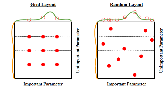
Grid Search
GridSearchCV: estimator, param_grid, cv
from sklearn.model_selection import GridSearchCV

params = [{"max_depth":[10, 20, 30],
           "max_features":[0.3, 0.5, 0.9]}]

# grid search
clf = GridSearchCV(RandomForestRegressor(), params, cv=3, n_jobs=-1)
clf.fit(X_train, y_train)
print("best values: ", clf.best_estimator_)
print("best score: ", clf.best_score_)

# final evaluation on test data
score = clf.score(X_test, y_test)
print("final score: ", score)

'''
best values:  RandomForestRegressor(max_depth=30, max_features=0.9)
best score:  0.9464442332854327
final score:  0.9589943180667339
'''
Randomized Search
RandomizedSearchCV: estimator, param_distributions, cv
from sklearn.model_selection import RandomizedSearchCV

n_estimators = [int(x) for x in np.linspace(start = 200, stop = 2000, num = 10)]
max_features = ['log2', 'sqrt']
max_depth = [int(x) for x in np.linspace(10, 110, num = 11)]
max_depth.append(None)
min_samples_split = [2, 5, 10]
min_samples_leaf = [1, 2, 4]
bootstrap = [True, False]

random_grid = {'n_estimators': n_estimators,
               'max_features': max_features,
               'max_depth': max_depth,
               'min_samples_split': min_samples_split,
               'min_samples_leaf': min_samples_leaf,
               'bootstrap': bootstrap}

rf = RandomizedSearchCV(RandomForestRegressor(), random_grid,
                               cv = 3, n_jobs = -1)
# Fit the random search model
rf.fit(X_train, y_train)

print(rf.best_params_, rf.best_estimator_, rf.best_score_)
score = rf.score(X_test, y_test)
print('final score:', score)

'''
{'n_estimators': 200, 'min_samples_split': 5, 'min_samples_leaf': 2, 'max_features': 'log2', 'max_depth': None, 'bootstrap': False} RandomForestRegressor(bootstrap=False, max_features='log2', min_samples_leaf=2,
                      min_samples_split=5, n_estimators=200) 0.9162766832621637
final score: 0.9365843295319143
'''
Leave a comment