[Machine Learning] Linear Classification

Linear classification (use Cross Entropy as loss function)

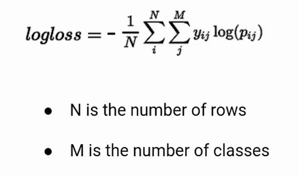
• also called log loss (logistic regression)
• Logistic Regression
• Classification by Calculating parameters one by one

Cross Entropy 손실 함수는 분류에 있어 기본적으로 많이 사용되는 손실 함수이고, 이진 분류에 사용되는 것을 Binary Cross Entropy 함수라고 합니다.

Cross Entropy

Binary Cross Entropy

Make dataset

make_blobs 함수를 사용하면 선형 분류에 적합한 데이터셋을 생성할 수 있습니다.

from sklearn.datasets import make_blobs

N = 500
(X, y) = make_blobs(n_samples=N, n_features=2, centers=2, cluster_std=2.0, random_state=17)
x1, x2 = X[:,0], X[:,1]
plt.scatter(X[:,0], X[:,1], c=y)

y[:10]

array([0, 1, 0, 1, 1, 0, 0, 0, 1, 0])

Train

w1 = np.random.randn()
w2 = np.random.randn()
b  = np.random.randn() 

def sigmoid_activation(z):
    return 1.0 / (1 + np.exp(-z))

lossHistory = []
epochs = 500
alpha = 0.03

for epoch in np.arange(epochs):
    z = w1*x1 + w2*x2 + b
    
    y_hat = sigmoid_activation(z)       # prediction

    loss = -((y*np.log(y_hat) + (1-y)*np.log(1-y_hat))).mean()  # loss = cross entropy
    lossHistory.append(loss)
    
    dloss_dz = y_hat - y
    w1_deriv = dloss_dz * x1        # d(loss)/dw1 = d(loss)/dz * dz/dw1
    w2_deriv = dloss_dz * x2
    b_deriv = dloss_dz * 1
    
    w1 = w1 - (alpha * w1_deriv).mean()
    w2 = w2 - (alpha * w2_deriv).mean()
    b  = b  - (alpha * b_deriv).mean()
    
    if epoch %10 == 0:
        print('epoch=', epoch, 'loss=', loss, 'w1=', w1, 'w2=', w2, 'b=', b)
    
    

print(w1, w2, b)
accuracy = ((sigmoid_activation(w1*x1 + w2*x2 + b) > 0.5) == y).sum()/N
print(accuracy)

# construct a figure that plots the loss over time
fig = plt.figure()
plt.plot(np.arange(0, epochs), lossHistory)
fig.suptitle("Training Loss")
plt.xlabel("Epoch #")
plt.ylabel("Loss")
plt.show()

epoch= 0 loss= 1.616035162169675 w1= -0.9490649093578043 w2= -0.49682963524704316 b= -0.696164229287423
epoch= 10 loss= 0.7008286524955278 w1= -0.4496766747447769 w2= -0.5260477241204355 b= -0.809026252878777
epoch= 20 loss= 0.29203905527389645 w1= -0.12827521312304996 w2= -0.5202691401157856 b= -0.8821467316261569
epoch= 30 loss= 0.1898689054567451 w1= 0.027749581072294832 w2= -0.5269227722920128 b= -0.9228796002094153
...
epoch= 490 loss= 0.09888960631144601 w1= 0.3732138813234712 w2= -1.0025023543610019 b= -1.4794882446903452

0.3732098201390971 -1.004432647797522 -1.4881961572489584
0.972

Plotting

plt.scatter(X[:,0], X[:,1], c=y)
xx = np.linspace(-10,10,100)
yy = -w1/w2 * xx -b/w2
plt.plot(xx, yy)
plt.show()

​

Linear classification (use Hinge loss as loss function)

• Hinge loss is primarily used with Support Vector Machine (SVM) Classifiers with class labels -1 and 1. So make sure you change the label of the ‘Malignant’ class in the dataset from 0 to -1.
• Hinge Loss not only penalizes the wrong predictions but also the right predictions that are not confident.
• Hinge loss for input-output pair (x,y) is given as:
  • L = max(0, 1 - yf(x))
  • L = 0 (if yf(x) >= 1), 1-yf(x) (otherwise)
  • dL/dw1 = 0 (if yf(x) >= 1), -yx1 (otherwise)

Make dataset

N = 500
(X, y_org) = make_blobs(n_samples=N, n_features=2, centers=2, cluster_std=2.0, random_state=17)
x1, x2 = X[:,0], X[:,1]
y = y_org.copy()
y[y==0] = -1
X[:5], y[:5], y_org[:5]

(array([[ -5.48619226,   1.21306671],
        [ -2.89056798,  -9.18025054],
        [ -1.5288614 ,   1.01129561],
        [ -7.48266658,  -9.99569036],
        [ -7.03983988, -10.35802726]]),
 array([-1,  1, -1,  1,  1]),
 array([0, 1, 0, 1, 1]))

Train

w1, w2, b = np.random.randn(), np.random.randn(), np.random.randn()
lossHistory = []
epochs = 500
alpha = 0.03

N = len(x1)
for epoch in np.arange(epochs):

    w1_deriv, w2_deriv, b_deriv, loss = 0., 0., 0., 0.
    for i in range(N):
        score = y[i]*(w1*x1[i] + w2*x2[i] + b)
        if score <= 1: # Loss 발생
            w1_deriv = w1_deriv - x1[i]*y[i]
            w2_deriv = w2_deriv - x2[i]*y[i]
            b_deriv = b_deriv - y[i]
            loss = loss + (1 - score)
        # else : derivatives are zero. loss is 0
    
    # mean
    w1_deriv /= float(N)
    w2_deriv /= float(N)
    b_deriv  /= float(N)
    loss /= float(N)
    # update parameters
    w1 = w1 - alpha * w1_deriv
    w2 = w2 - alpha * w2_deriv
    b  =  b - alpha *  b_deriv

    lossHistory.append(loss)
    
    if epoch %10 == 0:
        print('epoch=', epoch, 'loss=', loss, 'w1=', w1, 'w2=', w2, 'b=', b)
    
print(w1, w2, b)

accuracy = ((w1*x1 + w2*x2 + b > 0) == y_org).sum()/N
print(accuracy)

plt.plot(lossHistory)

epoch= 0 loss= 0.32953561452982716 w1= 0.10905148299148527 w2= -0.8707142547367681 b= -0.22266410994705235
epoch= 10 loss= 0.17294512065349388 w1= 0.2884756613203777 w2= -0.7980926952950345 b= -0.27570410994705236
epoch= 20 loss= 0.13295245866300887 w1= 0.3661718550159059 w2= -0.748069760577352 b= -0.3095441099470523
epoch= 30 loss= 0.12799019301386722 w1= 0.38203122269240997 w2= -0.7288418002221119 b= -0.33294410994705237
...
epoch= 490 loss= 0.06746119518336888 w1= 0.10373983094412123 w2= -0.46597462545524376 b= -1.144804109947046

0.1017903110742461 -0.4643184786720022 -1.1584841099470464
0.984

Training Loss

Plotting

plt.ylim([-15.,5.])
plt.scatter(X[:,0], X[:,1], c=y)

w1, w2, b = clf.coef_[0,0], clf.coef_[0,1], clf.intercept_
xx = np.linspace(-15,5,100)
yy = -w1/w2 * xx -b/w2
plt.plot(xx, yy, c='r')

Use library function

선형 분류를 위한 대표적인 분류 모델에는 SGDClassifier와 LogisticRegression 모델이 있습니다.

SGDClassifier 모델은 기본 손실 함수로 Hinge loss를 사용합니다.

LogisticRegression 모델은 기본 손실 함수로 Cross Entropy를 사용합니다.

from sklearn.linear_model import SGDClassifier, LogisticRegression
from sklearn.datasets import make_blobs

# Make dataset
N = 500
(X, y) = make_blobs(n_samples=N, n_features=2, centers=2, cluster_std=2.0, random_state=17)

# Create model and train
clf = SGDClassifier()      
clf.fit(X[:,:2], y)    
print("SGDClassifier: ", clf.score(X[:, :2],y))
print(clf.coef_, clf.intercept_)

log = LogisticRegression()      
log.fit(X[:,:2], y)    
print("Logistic Regression: ", log.score(X[:, :2],y))
print(log.coef_, log.intercept_)
plt.ylim([-15.,5.])
plt.scatter(X[:,0], X[:,1], c=y)

# Plotting
w1, w2, b = clf.coef_[0,0], clf.coef_[0,1], clf.intercept_
xx = np.linspace(-15,5,100)
yy = -w1/w2 * xx -b/w2
plt.plot(xx, yy, c='r')

w1, w2, b = log.coef_[0,0], log.coef_[0,1], log.intercept_
xx = np.linspace(-15,5,100)
yy = -w1/w2 * xx -b/w2
plt.plot(xx, yy, c='b')

SGDClassifier:  0.984
[[ -8.56625092 -34.52822982]] [-211.3932073]
Logistic Regression:  0.994
[[-0.46621709 -1.9549905 ]] [-10.32380395]